Introduction
While the devil is in the details, there are broadly two ways to go about building a scalable geospatial analytics engine.
One is to write something that natively understands geospatial analytics, has specialized handling for geospatial indices and geospatial queries.
The other is to take a general purpose distributed processing engine and specialize it for geospatial processing.
One of my goals in writing Magellan was to show that "one size fits all" does indeed work for geospatial analytics at scale. That is, it is possible to take a general purpose query processing framework and adapt it for geospatial analytics and still achieve state of the art in geospatial query performance.
I chose Spark as the general purpose engine for two reasons: Spark's performance, maturity and adoption meant most if not all big data processing over time would move to Spark, making it easy to integrate geospatial analytics with the rest of the ETL/ analytics pipelines.
The other is Spark's Catalyst optimizer. Catalyst is the powerful, extensible optimizer at the heart of Spark SQL. Its extensibility is what allows Magellan to be written on top of Spark and still leverage all the benefits that the core engine provides like join reordering, cost based optimization, efficient memory layout, whole stage code generation etc.
While the journey is not complete yet, Magellan is at a point where it performs very well on geospatial analytics on large datasets. We can easily scale spatial joins to billions of points and hundreds of thousands of shapes on commodity hardware on modest clusters and have it execute in under a couple of minutes. That is some serious scale and performance!
In this blog post, we will take a peek under the hood of Magellan to understand how it operates at scale.
Preliminaries
For the rest of this article, I am going to assume you are running an Apache Spark 2.2 cluster and Magellan version [1.0.5+].
We will be working with the NYC Taxicab dataset.
We will also use three different polygon datasets:
| Dataset | Number of Polygons | Avg # of edges per polygon |
|---|---|---|
| NYC Neighborhoods | 310 | 104 |
| NYC Census Blocks | 39192 | 14 |
| NY Census Blocks | 350169 | 51 |
The Join revisited
In the previous blog post, we were discussing a geospatial join of the form:
    val joined = trips.join(neighborhoods)
        .where($"point" within $"polygon")
Joining roughly O(200 million) points with the NYC Neighborhood dataset takes about 6 min on a 5 node r3 x.large cluster, as discussed before.
What we did not consider previously was the question: how does the time consumed in this join depend on the size of the polygon dataset?
Redoing the analysis of the previous blog post on all three polygon datasets with the exact same cluster and Spark configuration gives us a better picture:
| Dataset | Time taken (min) |
|---|---|
| NYC Neighborhoods | 6 |
| NYC Census Blocks | 840 |
| NY Census Blocks | > 4 days |
This is to be expected: the total time taken for the join is roughly proportional to the number of polygons in the dataset.
In the case of the naive join, the best we can do is to look at the bounding box of each polygon to decide whether a particular point has a chance of being inside. If the point is within the bounding box, we need to perform an expensive point in polygon test to determine if the point is actually inside the polygon.
Now that we have seen how the naive join works, let us do something less naive. Re run the analysis but before that, inject the following piece of code at the beginning:
magellan.Utils.injectRules(spark)
and provide a hint during the creation of the polygon dataframe what the index precision should be via:
spark.read.format("magellan").load($"path").index(30)
| Dataset | Time taken (min) (5 x r3.xlarge) | Time taken (min) (5 x c3.4xlarge) |
|---|---|---|
| NYC Neighborhoods | 1.6 | 0.5 |
| NYC Census Blocks | 3.5 | 0.9 |
| NY Census Blocks | 5.2 | 1.7 |
Ok, this is much better: the time taken for the computation is nearly independent of the size of the polygon dataset, over a three order of magnitude scale in the size of the polygon dataset
So, what happened?
Briefly, Magellan injects a Spatial Join Rule into Catalyst, which ends up building spatial indices on the fly for both the point and polygon datasets. The join is then rewritten under the hood to use these indices and avoid an expensive cartesian join in the first place.
The index precision provided as hint to the data frame via dataframe.index(precision) controls the granularity of the index.
To understand this better, let's start with how the point in polygon test works.
Point in Polygon Test
The basic problem we need to solve is: given a point and a polygon, how can we tell if the point is within the polygon or not?
There are many ways to solve this problem but perhaps the simplest is the so called ray casting algorithm.
The idea is very simple: Consider the polygon below, and two points, the red one outside the polygon and the blue one inside the polygon.
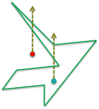
If we draw a ray from each point going out to infinity, the ray emanating from the point inside the polygon has to cross the polygon an odd number of times to escape, whereas the ray from the point outside has to cross an even number of times to escape.
So, by counting edge crossing modulo 2, we can determine if a point lies within the polygon or not.
If the number of edges of the polygon is p, the computational complexity of this algorithm is O(p).
Without precomputing anything, and for a generic (non convex) polygon, the worst case complexity of the point in polygon test is also O(p) so to do better than the algorithm above, we either need convexity or we need the ability to precompute stuff about the polygon so that at query time we do less computation.
Convexity is usually not under our control, so the next best thing is to see what we can precompute in order to simplify the problem.
The first thing we can do is given a polygon, precompute the bounding box, ie. the smallest axis parallel rectangle that encloses the polygon.
Once this is done, every time we need to check if a point is within the polygon, we first check if the point is within the bounding box. If not, we know for sure the point cannot be within the polygon.
If the point is within the bounding box, we proceed to do the more expensive point in polygon test to check if the point is actually inside the polygon.
This is an attractive solution because in the best case scenario, it avoids doing the expensive O(p) computation.
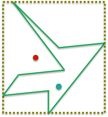
However, there are many scenarios where this still leads to more computation than necessary. In fact, the example below is a scenario where both the red and blue point would be inside the bounding box and would be indistinguishable unless a further test was applied.
There is another more subtle issue with using bounding boxes. Suppose you have m points and n polygons and you want to know for each point which polygon it falls into. For each polygon, you also know its bounding box.
Without looking at each bounding box for every given point, you cannot a priori conclude if a point falls inside a bounding box or not.
This means, knowing the bounding box of a polygon doesn't help you localize the tests to only points that are nearby in some sense and avoid the O(mn) computations.
Geospatial Indices
What if we knew that the set of all polygons were bounded by some large (but finite) bounding box?
In this case, you can further sub divide the bounding box into small enough cells and for each cell determine if the cell is either within, or overlaps or is disjoint from the polygon.
Similarly, for each point, you can determine which cell it falls inside.
Knowing which cell a point falls inside now allows us to prune all the polygons that do not contain/ or overlap that cell.
Furthermore, for polygons that contain that cell, we know for sure that the point is also within the polygon.
So the expensive point in polygon test needs to only be applied for the cells that overlap/ but are not contained in the polygon.
This in essence is the algorithm that Magellan employs.
There are many ways to construct these "cells". One approach is the so called Space Filling Curves. Magellan has an abstraction for constructing arbitrary types of space filling curves, though the implementation we support currently is the so called Morton Curve.
Leveraging Catalyst
The last piece of the puzzle is to transparently create and use these space filling curves as indices behind the scenes.
This is one of the places where Magellan leverages Catalyst's extensibility.
When Catalyst sees a join of the form
point.join(polygon).where($"point" within $"polygon")
it does not know what points and polygons mean: in particular that these are geometries.
However, it parses this data frame query and passes it through a pipeline of optimizations as below:
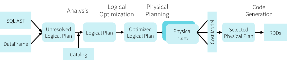
During construction of this pipeline there are various stages where external optimizations can be added. For example, additional analyzer rules, or optimizer rules or even rules affecting physical planning can be inserted into the Catalyst optimizer.
The plan that Magellan receives at the end of the optimization phase looks something like this:
![]()
The plan has resolved all variables, has pushed filters down as far as possible but beyond that there is nothing more that Catalyst can do as it is not aware of the nature of the data.
Magellan intercepts this plan and rewrites it to the following:
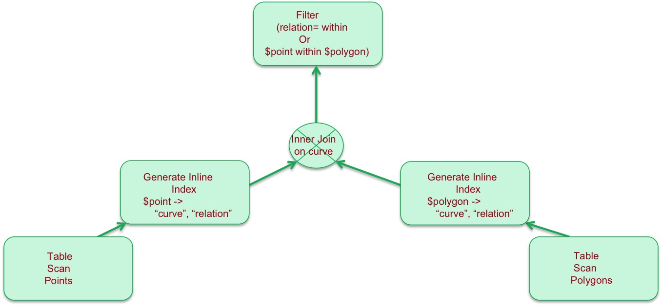
The rewritten plan includes an operator for each side of the join that takes the shape, computes the index and generates tuples of the form (shape, curve, relation) on either side of the join.
The curve represents the space filling curve of a given resolution while the relation represents how the curve relates to the geometry: is it within, overlapping or disjoint from the geometry.
The Join itself is rewritten to use the curve as key, while the filter is augmented with a condition that first checks if the curve is contained within the polygon in which case it short circuits the point in polygon test.
As this is all done under the hood, the user is able to automatically leverage new spatial join optimizations that Magellan adds without having to rewrite their code.
This blog post touched upon how Magellan scales geospatial queries and provided a peek under the hood of the Magellan engine.
You can also learn more about Magellan from the following:
- Magellan project on GitHub
- The slides for my Spark Summit Europe 2016 talk on Magellan
- My talk at Foss4g where I presented some results of benchmarking Magellan on a single node and compared other geospatial libraries on big data.
- My Strata 2018 Slides on Magellan, outlining its current performance, the architecture etc.